Using the picasso trained predictors#
This notebook shows how one can use the trained models to make predictions of gas thermodynamics from halo properties. For a full documentation of the predictor objects and their methods, see picasso.predictors: From halo properties to gas properties.
import jax
import jax.numpy as jnp
import matplotlib.pyplot as plt
import pandas as pd

from picasso import predictors
from picasso.test_data import halos, profs

import seaborn as sns

sns.set_style("darkgrid")
sns.set_theme("notebook")

benchmark = True
We will use the minimal_576 trained model, which takes as input halo mass and concentration:
predictor = predictors.minimal_576
print(predictor.input_names)
['log M200' 'c200']
Predicting gas model parameters#
First, we want to compute predictions for the model parameter vector, \(\vartheta_{\rm gas}\). To do so, we simply need the vector of scalar halo properties \(\vartheta_{\rm halo}\). We’ll use some pre-stored data (containing four halos from the simulations presented in Kéruzoré+24) and write the input vector:
logM200c = halos["log M200"]
c200c = jnp.array(halos["c200"])
theta_halo = jnp.array([logM200c, c200c]).T
print(theta_halo.shape)
(7, 2)
We can then use the predictor.predict_model_parameters() function to predict \(\vartheta_{\rm gas}\). For a single halo:
theta_gas_0 = predictor.predict_model_parameters(theta_halo[0])
print(theta_gas_0)
[ 2.8579862   1.5800635   1.1345413   0.          0.76251674 -1.3342006
 -0.5730133   0.8244546 ]
Note that the predictors have been trained in log-space for some of the parameters, and make their predictions in that space. The exact normalization of the predictions is that of Table 1 in the paper:
Symbol |
Meaning |
Range |
|---|---|---|
\(\log_{10} \rho_0\) |
(log-scaled) Central normalized gas density |
\((1.5, \, 5)\) |
\(\log_{10} P_0\) |
(log-scaled) Central normalized gas total pressure |
\((0, \, 4.5)\) |
\(\Gamma_0\) |
Gas polytropic index limit as \(r \rightarrow \infty\) |
\((1, \, 1.4)\) |
\(c_\gamma\) |
Gas polytropic index shape parameter |
\([0]\)* |
\(\theta_0 / (10^{-6} \, {\rm km^2 s^{-2}})\) |
Polytropic normalization |
\((0, \, 2)\) |
\(\log_{10} A_{\rm nt}\) |
(log-scaled) Central plateau of non-thermal pressure fraction |
\((-4, \, 0)\) |
\(\log_{10} B_{\rm nt}\) |
(log-scaled) Non-thermal pressure fraction at \(r=2R_{500c}\) |
\((-1.5, \, 0)\) |
\(C_{\rm nt}\) |
Non-thermal pressure fraction profile power law index |
\((0, \, 4)\) |
* \((-1,\, 1)\) for the NR+\(\Gamma(r)\) and SG+\(\Gamma(r)\) models.
The predictor.predict_model_parameters() function can also be used for several halos at a time:
theta_gas = predictor.predict_model_parameters(theta_halo)
print(f"{theta_gas=}")
print(f"{theta_gas.shape=}")
theta_gas=Array([[ 2.8579862 ,  1.5800636 ,  1.1345413 ,  0.        ,  0.7625168 ,
        -1.3342004 , -0.5730133 ,  0.8244548 ],
       [ 3.0891585 ,  1.8412256 ,  1.1362435 ,  0.        ,  0.49745762,
        -1.423728  , -0.56955934,  1.0702431 ],
       [ 3.0761304 ,  1.8216532 ,  1.1312138 ,  0.        ,  0.3338053 ,
        -1.3907712 , -0.5089177 ,  1.0523993 ],
       [ 2.8483396 ,  1.5602771 ,  1.1200436 ,  0.        ,  0.24938817,
        -1.3459554 , -0.46140385,  0.853472  ],
       [ 2.9394426 ,  1.6772497 ,  1.1291878 ,  0.        ,  0.16645454,
        -1.3711526 , -0.45240808,  0.94847983],
       [ 2.9498107 ,  1.6725324 ,  1.1352186 ,  0.        ,  0.1211944 ,
        -1.3999796 , -0.4420457 ,  1.0124265 ],
       [ 3.2267897 ,  2.0133085 ,  1.1500207 ,  0.        ,  0.07647304,
        -1.5900545 , -0.49178195,  1.3881102 ]], dtype=float32)
theta_gas.shape=(7, 8)
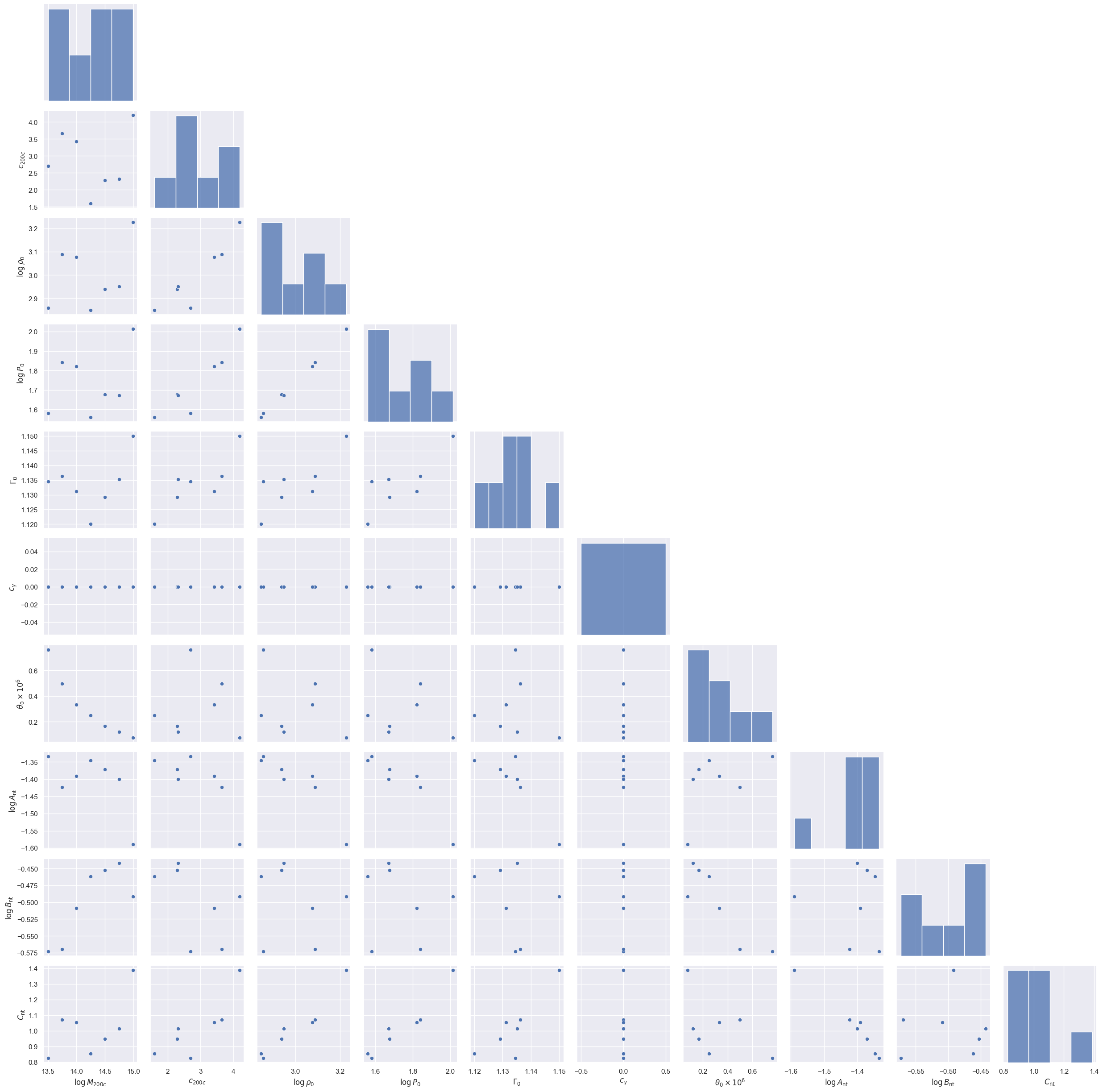
df = {"$\\log M_{200c}$": logM200c, "$c_{200c}$": c200c}
for i, name in enumerate(
    [
        "$\\log \\rho_0$",
        "$\\log P_0$",
        "$\\Gamma_0$",
        "$c_\\gamma$",
        "$\\theta_0 \\times 10^6$",
        "$\\log A_{\\rm nt}$",
        "$\\log B_{\\rm nt}$",
        "$C_{\\rm nt}$",
    ]
):
    df[name] = theta_gas[:, i]
df = pd.DataFrame(df)

pg = sns.PairGrid(df, corner=True, diag_sharey=False)
pg.map_lower(sns.scatterplot)
pg.map_diag(sns.histplot)
<seaborn.axisgrid.PairGrid at 0x31e7e9f70>
It can also be just-in-time compiled:
if benchmark:
    predict_jit = jax.jit(predictor.predict_model_parameters)
    print("Not jitted:", end=" ")
    %timeit _ = predictor.predict_model_parameters(theta_halo)
    print("jitted:", end=" ")
    _ = predict_jit(theta_halo)
    %timeit _ = predict_jit(theta_halo)
Not jitted: 5.76 ms ± 80.5 μs per loop (mean ± std. dev. of 7 runs, 100 loops each)
jitted: 13.9 μs ± 423 ns per loop (mean ± std. dev. of 7 runs, 100,000 loops each)
Predicting gas thermodynamics#
With a prediction for \(\vartheta_{\rm gas}\), we can use picasso.polytrop and picasso.nonthermal to predict gas thermodynamics (see Using the picasso analytical gas model).
PicassoPredictor objects also offers a wrapper function that predicts all thermodynamic properties directly from an input vector \(\vartheta_{\rm halo}\) and a potential distribution.
Assuming the halos above are NFW, we can predict their potential profiles:
r_R500c, phi = profs["r_R500"], profs["phi"]
Then, we can make predictions of gas thermodynamics for one halo:
rho_g, P_tot, P_th, f_nt = predictor.predict_gas_model(
    theta_halo[0], phi[0], r_R500c[0], r_R500c[0] / 2
)
Or for all halos at the same time (this function uses jax.vmap to vectorize the predictions):
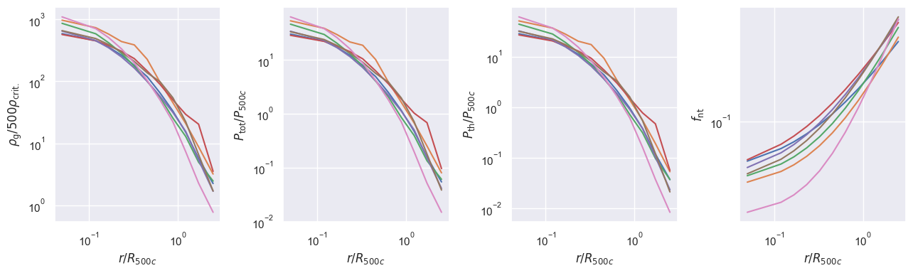
rho_g, P_tot, P_th, f_nt = predictor.predict_gas_model(
    theta_halo, phi, r_R500c, r_R500c / 2
)
fig, axs = plt.subplots(1, 4, figsize=(13, 4))
for ax, q in zip(axs, [rho_g, P_tot, P_th, f_nt]):
    ax.loglog(r_R500c.T, q.T)
    ax.set_xlabel("$r / R_{500c}$")

axs[0].set_ylabel("$\\rho_{\\rm g} / 500 \\rho_{\\rm crit.}$")
axs[1].set_ylabel("$P_{\\rm tot} / P_{500c}$")
axs[2].set_ylabel("$P_{\\rm th} / P_{500c}$")
axs[3].set_ylabel("$f_{\\rm nt}$")
fig.tight_layout()
Again, these functions can be just-in-time compiled:
if benchmark:
    predict_jit = jax.jit(predictor.predict_gas_model)

    print("1 halo, not jitted:", end=" ")
    %timeit _ = predictor.predict_gas_model(theta_halo[0], phi[0], r_R500c[0], r_R500c[0] / 2)
    print("1 halo, jitted:", end=" ")
    _ = predict_jit(theta_halo[0], phi[0], r_R500c[0], r_R500c[0] / 2)
    %timeit _ = predict_jit(theta_halo[0], phi[0], r_R500c[0], r_R500c[0] / 2)

    print("4 halo, not jitted:", end=" ")
    %timeit _ = predictor.predict_gas_model(theta_halo, phi, r_R500c, r_R500c / 2)
    print("4 halo, jitted:", end=" ")
    _ = predict_jit(theta_halo, phi, r_R500c, r_R500c / 2)
    %timeit _ = predict_jit(theta_halo, phi, r_R500c, r_R500c / 2)
1 halo, not jitted: 7.55 ms ± 185 μs per loop (mean ± std. dev. of 7 runs, 100 loops each)
1 halo, jitted: 188 μs ± 4.17 μs per loop (mean ± std. dev. of 7 runs, 10,000 loops each)
4 halo, not jitted: 13.3 ms ± 216 μs per loop (mean ± std. dev. of 7 runs, 100 loops each)
4 halo, jitted: 47.3 μs ± 2.43 μs per loop (mean ± std. dev. of 7 runs, 10,000 loops each)
For an example of how these predictions can be included in a differentiable loss function and used to train a picasso model, see Training a picasso predictor.