Using the picasso analytical gas model

This notebook shows how one can use the picasso.polytrop and picasso.nonthermal modules to compute gas properties from a gravitational potential distribution. For a full documentation of the functions available in both modules, see picasso.polytrop: Polytropic gas model and picasso.nonthermal: Non-thermal pressure support.

import jax
import jax.numpy as jnp
import matplotlib.pyplot as plt

from picasso import polytrop, nonthermal
from picasso.test_data import halos, profs

import seaborn as sns

sns.set_style("darkgrid")
sns.set_theme("notebook")

benchmark = True

The analytical gas model

The polytropic gas model can be written as (see Kéruzoré+24):

\[\begin{split} \rho(\phi, \, r) = \rho_0 \theta^{\Gamma(r) / (\Gamma(r) - 1)}(\phi), \\[10pt] P(\phi, \, r) = P_0 \theta^{1 / (\Gamma(r) - 1)}(\phi), \end{split}\]

where \(\phi\) is the halo’s gravitational potential, and $\( \theta(\phi) = 1 - \theta_0 (\phi - \phi_0), \)$

The gas polytropic index, \(\Gamma\), is allowed to vary with radius as:

\[\begin{split} \Gamma(r) = \begin{cases} \begin{aligned} & \; 1 + (\Gamma_0 - 1) \frac{1}{1 + e^{-x}} & c_\Gamma > 0; \\ & \; \Gamma_0 & c_\Gamma = 0; \\ & \; \Gamma_0 + (\Gamma_0 - 1) \left(1 - \frac{1}{1 + e^{x}}\right) & c_\Gamma < 0, \\ \end{aligned} \end{cases} \end{split}\]

with \(x \equiv r / (c_\gamma R_{500c})\).

This model has five parameters: \((\rho_0, P_0)\) are the central value of gas density and pressure, \(\Gamma_0\) is the asymptotic value of the polytropic index as \(r \rightarrow \infty\), \(c_\gamma\) is the polytropic concentration (\(c_\gamma = 0\) implies \(\Gamma(r) = \Gamma_0\)), and \(\theta_0\) is a shape parameter.

We further write the fraction of non-thermal pressure as a power-law of radius, plus a constant plateau:

\[ f_{\rm nt}(r) = A_{\rm nt} + (B_{\rm nt} - A_{\rm nt}) \left(\frac{r}{2R_{500c}}\right)^{C_{\rm nt}} \]

This adds three parameters to our gas model: \(A_{\rm nt}\) is the central value of non-thermal pressure fraction, \(B_{\rm nt}\) is the non-thermal pressure fraction at \(r=2R_{500c}\), and \(C_{\rm nt}\) is the power law evolution with radius.

Halo potential and gas model parameters

Making predictions of gas properties using this model requires two ingredients: a potential distribution, and a vector containing values for the eight parameters of the gas model, \(\vartheta_{\rm gas}\). The picasso model is based on using a neural network to predict the latter (see Using the picasso trained predictors); here, we are interested in using the gas model independently, assuming we independently obtained a prediction of the vector parameter.

We will use simple NFW halos to make predictions. We’ll use some pre-stored data (containing mass and concentration values for four halos from the simulations presented in Kéruzoré+24) and compute their potential profiles:

phi, r_R500c = profs["phi"], profs["r_R500"]

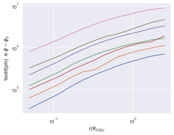
Note that, as stated in the paper, the code defines the potential phi as the normalized potential, \(\phi - \phi_0\), so phi should be 0 at the center of halos (potential minimum) and increase to plateau at a positive value at large radii:

fig, ax = plt.subplots()
ax.loglog(r_R500c.T, phi.T)
ax.set_xlabel("$r / R_{500c}$")
ax.set_ylabel("\\texttt{phi} $\\equiv \\phi - \\phi_0$")

Text(0, 0.5, '\\texttt{phi} $\\equiv \\phi - \\phi_0$')

For simplicity, we will use fixed values for the parameter vector \(\vartheta_{\rm gas}\):

# rho_0, P_0, Gamma_0, c_gamma, theta_0, A_nt, B_nt, C_nt
theta_gas = jnp.array(
    [3.22e3, 1.91e2, 1.134, 0.0, 3.594e-7, 1.18e-2, 2.11e-1, 1.647]
)

Polytropic model: density and total pressure

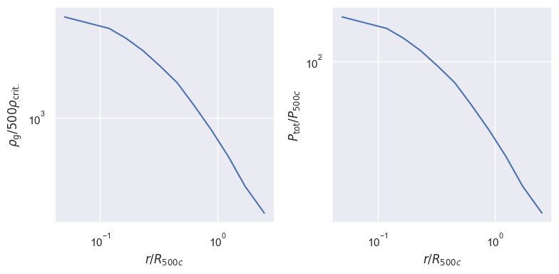
First, focusing on one halo, we can use polytrop.rho_P_g to compute density and total pressure:

rho_g, P_tot = polytrop.rho_P_g(phi[0], r_R500c[0], *theta_gas[:5])

fig, axs = plt.subplots(1, 2, figsize=(8, 4))
for ax, q in zip(axs, [rho_g, P_tot]):
    ax.loglog(r_R500c[0], q)
    ax.set_xlabel("$r / R_{500c}$")
axs[0].set_ylabel("$\\rho_{\\rm g} / 500 \\rho_{\\rm crit.}$")
axs[1].set_ylabel("$P_{\\rm tot} / P_{500c}$")
fig.tight_layout()

The function can easily be compiled just-in-time:

rho_P_g = jax.jit(polytrop.rho_P_g)
rho_g, P_tot = rho_P_g(phi[0], r_R500c[0], *theta_gas[:5])

if benchmark:
    print("Not jitted:", end=" ")
    %timeit _ = polytrop.rho_P_g(phi[0], r_R500c[0], *theta_gas[:5])
    print("jitted:", end=" ")
    %timeit _ = rho_P_g(phi[0], r_R500c[0], *theta_gas[:5])

Not jitted: 457 μs ± 2.08 μs per loop (mean ± std. dev. of 7 runs, 1,000 loops each)
jitted: 128 μs ± 989 ns per loop (mean ± std. dev. of 7 runs, 10,000 loops each)

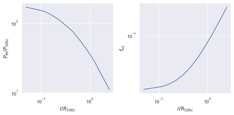
Non-thermal pressure fraction and thermal pressure

Similarly, the non-thermal pressure fraction can be computed using nonthermal.f_nt_generic, and be used to derive the thermal pressure:

f_nt = nonthermal.f_nt_generic(r_R500c[0] / 2, *theta_gas[5:])
P_th = P_tot * (1 - f_nt)

fig, axs = plt.subplots(1, 2, figsize=(8, 4))
for ax, q in zip(axs, [P_th, f_nt]):
    ax.loglog(r_R500c[0], q)
    ax.set_xlabel("$r / R_{500c}$")
axs[0].set_ylabel("$P_{\\rm th} / P_{500c}$")
axs[1].set_ylabel("$f_{\\rm nt}$")
fig.tight_layout()

These can also be compiled:

@jax.jit
def f_nt_and_P_th(*args):
    f_nt = nonthermal.f_nt_generic(*args)
    return f_nt, P_tot * (1 - f_nt)


_ = f_nt_and_P_th(r_R500c[0] / 2, *theta_gas[5:])

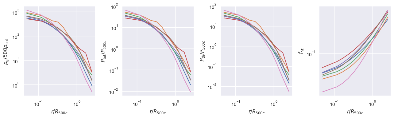
Batch predictions

The picasso.polytrop and picasso.nonthermal modules can also be used to make predictions for several halos at a time:

theta_gas = jnp.array(
    [
        [ 6.8168e02, 4.2554e01, 1.1553e00, 0.0000e00, 9.0783e-07, 4.2568e-02, 2.6434e-01, 8.6513e-01],
        [ 1.1593e03, 6.6720e01, 1.1435e00, 0.0000e00, 5.1063e-07, 3.7982e-02, 2.7196e-01, 1.0898e00],
        [ 1.1806e03, 6.6686e01, 1.1394e00, 0.0000e00, 3.4640e-07, 4.1790e-02, 3.0468e-01, 1.0849e00],
        [ 6.2562e02, 3.4515e01, 1.1449e00, 0.0000e00, 2.8243e-07, 4.9366e-02, 3.3784e-01, 8.4570e-01],
        [ 8.4713e02, 4.7153e01, 1.1409e00, 0.0000e00, 1.7668e-07, 4.3313e-02, 3.4503e-01, 9.4095e-01],
        [ 9.0735e02, 5.1616e01, 1.1423e00, 0.0000e00, 1.2721e-07, 4.0001e-02, 3.5159e-01, 9.7828e-01],
        [ 1.8332e03, 1.0815e02, 1.1419e00, 0.0000e00, 7.6836e-08, 2.4986e-02, 3.2474e-01, 1.3087e00],
    ]
)

We have to be a bit smart about array shapes here (or, alternatively, one may want to use jax.vmap):

def thermodynamics(phi, theta_gas, r_pol, r_fnt):
    rho_g, P_tot = polytrop.rho_P_g(
        phi,
        r_pol,
        theta_gas[..., 0, None],
        theta_gas[..., 1, None],
        theta_gas[..., 2, None],
        theta_gas[..., 3, None],
        theta_gas[..., 4, None],
    )
    f_nt = nonthermal.f_nt_generic(
        r_fnt,
        theta_gas[..., 5, None],
        theta_gas[..., 6, None],
        theta_gas[..., 7, None],
    )
    return rho_g, P_tot, P_tot * (1 - f_nt), f_nt


rho_g, P_tot, P_th, f_nt = thermodynamics(phi, theta_gas, r_R500c, r_R500c / 2)

fig, axs = plt.subplots(1, 4, figsize=(13, 4))
for ax, q in zip(axs, [rho_g, P_tot, P_th, f_nt]):
    ax.loglog(r_R500c.T, q.T)
    ax.set_xlabel("$r / R_{500c}$")

axs[0].set_ylabel("$\\rho_{\\rm g} / 500 \\rho_{\\rm crit.}$")
axs[1].set_ylabel("$P_{\\rm tot} / P_{500c}$")
axs[2].set_ylabel("$P_{\\rm th} / P_{500c}$")
axs[3].set_ylabel("$f_{\\rm nt}$")
fig.tight_layout()

Again, these functions can be compiled:

if benchmark:
    print("Not jitted:", end=" ")
    %timeit _ = thermodynamics(phi, theta_gas, r_R500c, r_R500c / 2)

    thermodynamics = jax.jit(thermodynamics)
    print("jitted:", end=" ")
    %timeit _ = thermodynamics(phi, theta_gas, r_R500c, r_R500c / 2)

Not jitted: 1.39 ms ± 11.2 μs per loop (mean ± std. dev. of 7 runs, 1,000 loops each)
jitted: 25.9 μs ± 1.45 μs per loop (mean ± std. dev. of 7 runs, 10,000 loops each)