Using the picasso trained predictors#
This notebook shows how one can use the trained models to make predictions of gas thermodynamics from halo properties. For a full documentation of the predictor objects and their methods, see picasso.predictors: From halo properties to gas properties.
import jax
import jax.numpy as jnp
import matplotlib.pyplot as plt
import pandas as pd

from picasso import predictors
from picasso.test_data import halos, profs

import seaborn as sns
sns.set_style("darkgrid")
sns.set_theme("notebook")

benchmark = True
---------------------------------------------------------------------------
ModuleNotFoundError                       Traceback (most recent call last)
Cell In[1], line 1
----> 1 import jax
      2 import jax.numpy as jnp
      3 import matplotlib.pyplot as plt

ModuleNotFoundError: No module named 'jax'
We will use the minimal_576 trained model, which takes as input halo mass and concentration:
predictor = predictors.minimal_576
print(predictor.input_names)
['log M200' 'c200']
Predicting gas model parameters#
First, we want to compute predictions for the model parameter vector, \(\vartheta_{\rm gas}\). To do so, we simply need the vector of scalar halo properties \(\vartheta_{\rm halo}\). We’ll use some pre-stored data (containing four halos from the simulations presented in Kéruzoré+24) and write the input vector:
logM200c = halos["log M200"]
c200c = jnp.array(halos["c200"])
theta_halo = jnp.array([logM200c, c200c]).T
print(theta_halo.shape)
(7, 2)
We can then use the predictor.predict_model_parameters() function to predict \(\vartheta_{\rm gas}\). For a single halo:
theta_gas_0 = predictor.predict_model_parameters(theta_halo[0])
print(theta_gas_0)
[ 2.9106064   1.6468848   1.1334685   0.          0.7579316  -1.3241944
 -0.5855      0.85590917]
The predictor.predict_model_parameters() function can also be used for several halos at a time:
theta_gas = predictor.predict_model_parameters(theta_halo)
print(f"{theta_gas=}")
print(f"{theta_gas.shape=}")
theta_gas=Array([[ 2.9106064 ,  1.6468848 ,  1.1334685 ,  0.        ,  0.7579316 ,
        -1.3241944 , -0.5855    ,  0.85590917],
       [ 3.0965114 ,  1.8520657 ,  1.1311967 ,  0.        ,  0.48492068,
        -1.4299242 , -0.5614897 ,  1.1043483 ],
       [ 3.0746489 ,  1.8180763 ,  1.1310333 ,  0.        ,  0.3356811 ,
        -1.37233   , -0.5092694 ,  1.0796801 ],
       [ 2.8056588 ,  1.5297322 ,  1.1362283 ,  0.        ,  0.27505645,
        -1.4245594 , -0.48284996,  0.7942678 ],
       [ 2.950333  ,  1.6717771 ,  1.1333015 ,  0.        ,  0.17360152,
        -1.400001  , -0.47301912,  0.89461106],
       [ 2.9969964 ,  1.7104851 ,  1.1341447 ,  0.        ,  0.12555973,
        -1.4094577 , -0.47190595,  0.9506246 ],
       [ 3.2324495 ,  2.008476  ,  1.1400145 ,  0.        ,  0.07529356,
        -1.5716207 , -0.50930977,  1.2982608 ]], dtype=float32)
theta_gas.shape=(7, 8)
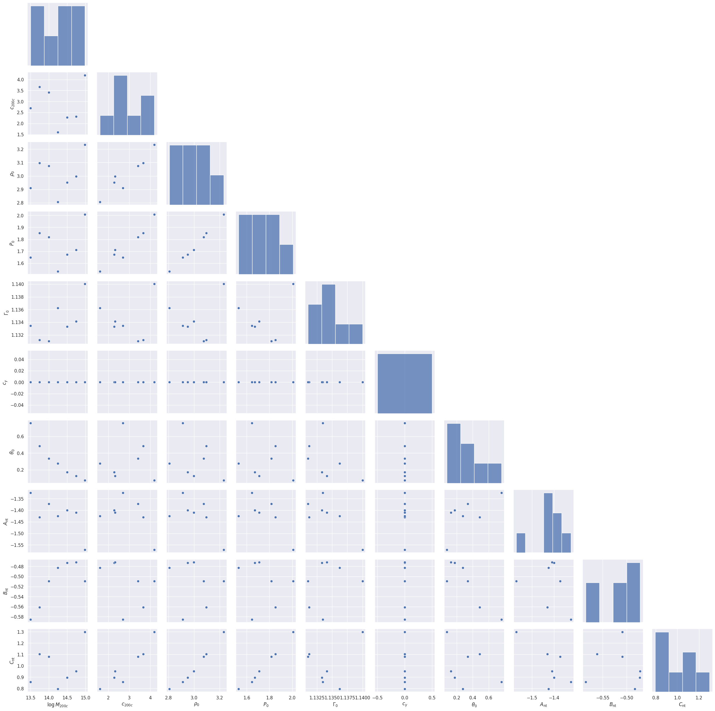
df = {"$\\log M_{200c}$": logM200c, "$c_{200c}$": c200c}
for i, name in enumerate(
    [
        "$\\rho_0$",
        "$P_0$",
        "$\\Gamma_0$",
        "$c_\\gamma$",
        "$\\theta_0$",
        "$A_{\\rm nt}$",
        "$B_{\\rm nt}$",
        "$C_{\\rm nt}$",
    ]
):
    df[name] = theta_gas[:, i]
df = pd.DataFrame(df)

pg = sns.PairGrid(df, corner=True, diag_sharey=False)
pg.map_lower(sns.scatterplot)
pg.map_diag(sns.histplot)
<seaborn.axisgrid.PairGrid at 0x7f92983da160>
It can also be just-in-time compiled:
if benchmark:
    predict_jit = jax.jit(predictor.predict_model_parameters)
    print("Not jitted:", end=" ")
    %timeit _ = predictor.predict_model_parameters(theta_halo)
    print("jitted:", end=" ")
    _ = predict_jit(theta_halo)
    %timeit _ = predict_jit(theta_halo)
Not jitted: 17 ms ± 212 µs per loop (mean ± std. dev. of 7 runs, 100 loops each)
jitted: 12.8 µs ± 998 ns per loop (mean ± std. dev. of 7 runs, 100,000 loops each)
Predicting gas thermodynamics#
With a prediction for \(\vartheta_{\rm gas}\), we can use picasso.polytrop and picasso.nonthermal to predict gas thermodynamics (see Using the picasso analytical gas model).
PicassoPredictor objects also offers a wrapper function that predicts all thermodynamic properties directly from an input vector \(\vartheta_{\rm halo}\) and a potential distribution.
Assuming the halos above are NFW, we can predict their potential profiles:
r_R500c, phi = profs["r_R500"], profs["phi"]
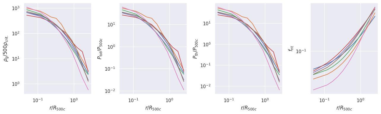
Then, we can make predictions of gas thermodynamics for one halo:
rho_g, P_tot, P_th, f_nt = predictor.predict_gas_model(theta_halo[0], phi[0], r_R500c[0], r_R500c[0] / 2)
Or for all halos at the same time (this function uses jax.vmap to vectorize the predictions):
rho_g, P_tot, P_th, f_nt = predictor.predict_gas_model(theta_halo, phi, r_R500c, r_R500c / 2)
fig, axs = plt.subplots(1, 4, figsize=(13, 4))
for ax, q in zip(axs, [rho_g, P_tot, P_th, f_nt]):
    ax.loglog(r_R500c.T, q.T)
    ax.set_xlabel("$r / R_{500c}$")

axs[0].set_ylabel("$\\rho_{\\rm g} / 500 \\rho_{\\rm crit.}$")
axs[1].set_ylabel("$P_{\\rm tot} / P_{500c}$")
axs[2].set_ylabel("$P_{\\rm th} / P_{500c}$")
axs[3].set_ylabel("$f_{\\rm nt}$")
fig.tight_layout()
Again, these functions can be just-in-time compiled:
if benchmark:
    predict_jit = jax.jit(predictor.predict_gas_model)

    print("1 halo, not jitted:", end=" ")
    %timeit _ = predictor.predict_gas_model(theta_halo[0], phi[0], r_R500c[0], r_R500c[0] / 2)
    print("1 halo, jitted:", end=" ")
    _ = predict_jit(theta_halo[0], phi[0], r_R500c[0], r_R500c[0] / 2)
    %timeit _ = predict_jit(theta_halo[0], phi[0], r_R500c[0], r_R500c[0] / 2)

    print("4 halo, not jitted:", end=" ")
    %timeit _ = predictor.predict_gas_model(theta_halo, phi, r_R500c, r_R500c / 2)
    print("4 halo, jitted:", end=" ")
    _ = predict_jit(theta_halo, phi, r_R500c, r_R500c / 2)
    %timeit _ = predict_jit(theta_halo, phi, r_R500c, r_R500c / 2)
1 halo, not jitted: 21.5 ms ± 296 µs per loop (mean ± std. dev. of 7 runs, 10 loops each)
1 halo, jitted: 376 µs ± 16.4 µs per loop (mean ± std. dev. of 7 runs, 1,000 loops each)
4 halo, not jitted: 38.8 ms ± 244 µs per loop (mean ± std. dev. of 7 runs, 10 loops each)
4 halo, jitted: 33.9 µs ± 772 ns per loop (mean ± std. dev. of 7 runs, 10,000 loops each)
For an example of how these predictions can be included in a differentiable loss function and used to train a picasso model, see Training a picasso predictor.